Thanks to Alex Cai for the discussion that inspired these ideas. Also, thanks to Stephen Casper for feedback.

In this post, I want to briefly cover the results of the 2017 paper “Universal adversarial perturbations”¹, and discuss what it implies about the geometry of classification boundaries. I hope to make this post accessible to readers who are new to machine learning, so I will not assume any prior knowledge beyond a general math background.

Neural Networks

Here’s my understanding of how (deep) neural nets work. Say we have a neural network that has been trained to classify images of a fixed size. That is, given an image of \(n \times m\) pixels, it assigns it to a class like “dog” or “pillow”. The network consists of a bunch of layers of nodes as shown below. On the very left, we have an input layer of \(3nm\) input nodes: one for each color channel (RGB) of each pixel in the image. In the middle, we have a bunch of “hidden layers,” and then on the right, we have an output layer that contains one node for each of the network’s classification options.

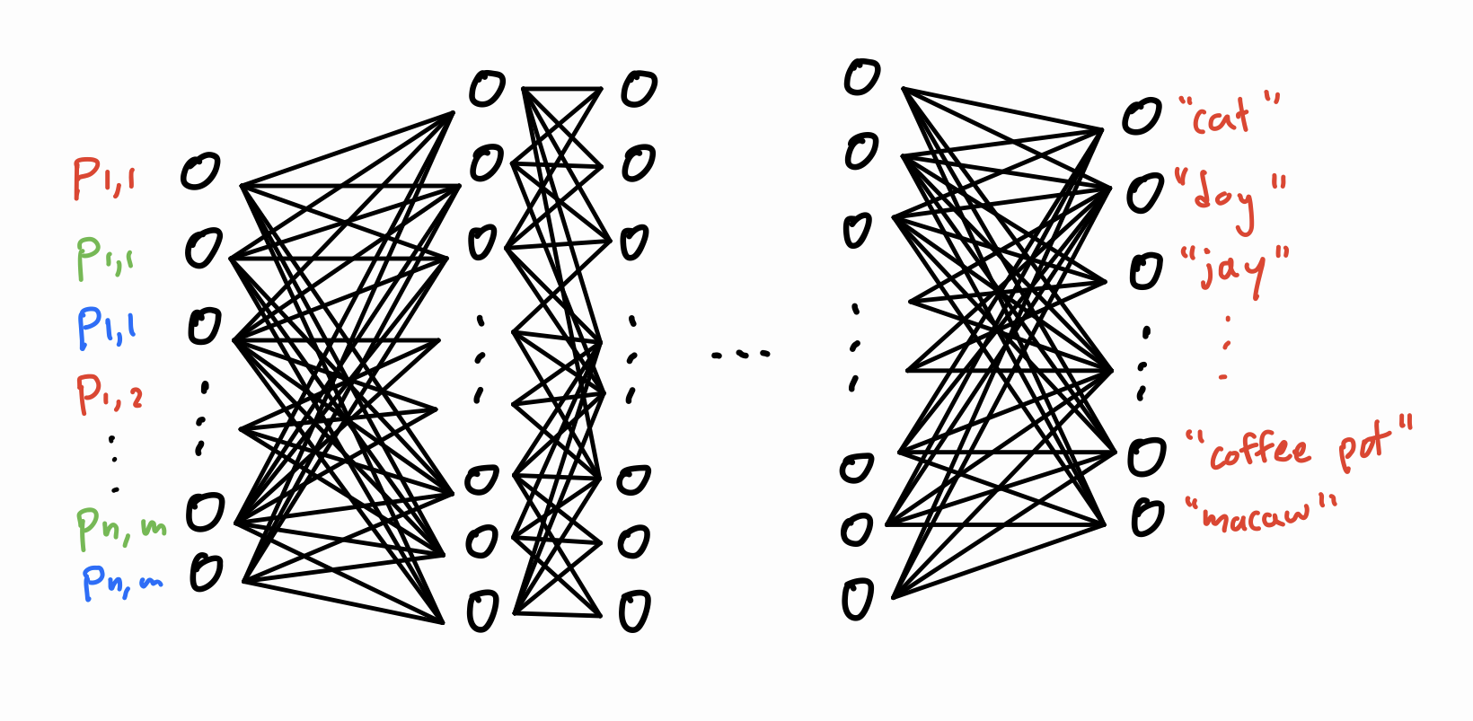
A rendition of a deep neural network.

We can feed an image into our neural net by setting the “activations” of the nodes in the input layer to the RGB values of the pixels of the image. Then, the activation of each node in a later layer is computed by taking a linear combination of node activations in the previous layer, then applying a simple nonlinear function such as sigmoid \((1 + \exp(-x))^{-1}\) or ReLU \(\frac{1}{2}(x + \lvert x \rvert)\). Once all of these activations are computed, the output layer tells us how likely the model thinks the image falls into each class, with the highest output activation representing its most predicted class.

Assuming that our model is already trained (that is, we’ve figured out good linear combinations to use for the node activations), the hope is that this final classification is correct for most images – even those that were not in the training set. Indeed, modern neural nets have been able to achieve very high classification accuracies. For this post, I’m going to assume that our model has near 100% accuracy on images in the test distribution \(D\). I will also use the words “model” and “neural network” interchangeably.

Adversarial Perturbations

The authors of this paper were able to find adversarial perturbations for state-of-the-art deep neural nets. Say that our network correctly classifies an image \(I\) as “coffeepot”. An adversarial perturbation is a small change \(\Delta\) such that the network classifies \(I' = I + \Delta\) as something else entirely, such as “macaw” (addition of images is done exactly how you would expect: add up the RGB values, pixel by pixel). Surprisingly, \(\Delta\) can be so small that it is barely perceptible to the human eye – they were able to find perturbations that changed the RGB color value of each pixel by at most \(10\) (on a scale from \(0\) to \(255\)).

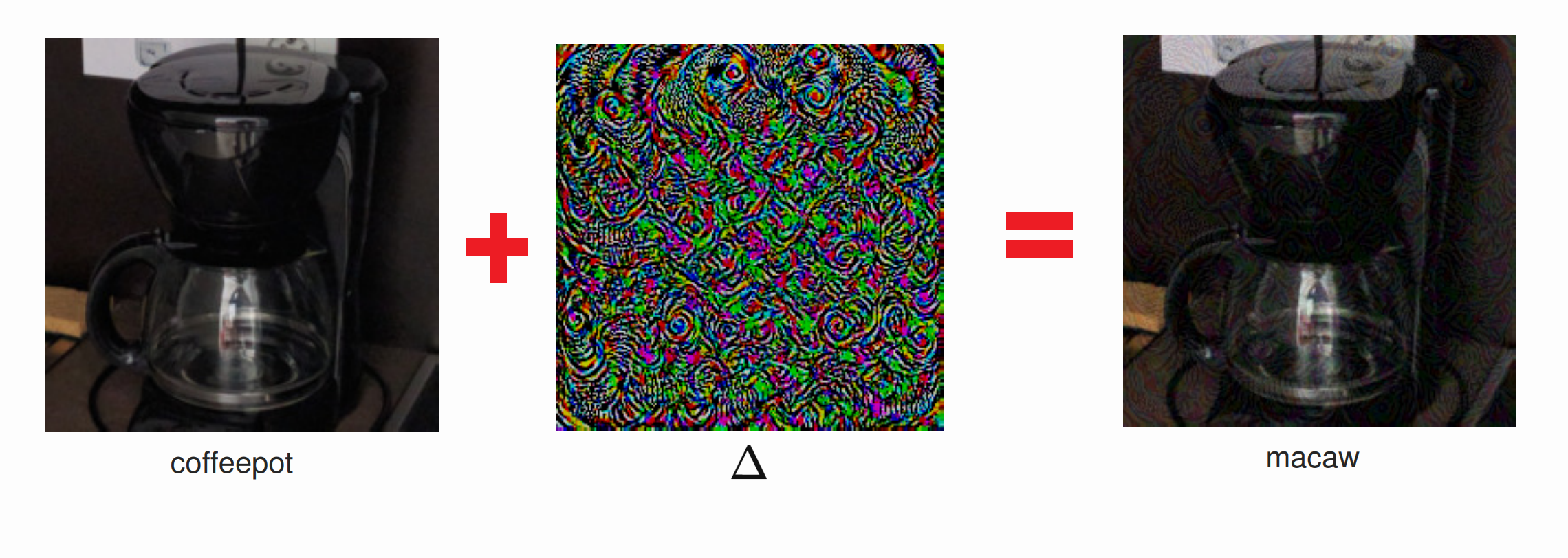
If you add a small perturbation to a normal image of a coffeepot, the neural network misclassifies it as a "macaw". The colors of the middle perturbation image have been scaled up for visibility.
Image credit: Moosavi-Dezfooli et al.

This points to a serious problem with our neural network that could lead to real-world failures. As an example, say that airports begin using deep neural nets to screen passport photos. This could be a security issue if terrorists were to modify their own photos with these adversarial perturbations, causing the network to fail to recognize them.

But it’s even worse. By default, there is no reason to expect that a perturbation \(\Delta\) that fools the network on a specific image will also fool the network when applied to other images. Surprisingly, the researchers were able to find some perturbations that were universal². That is, they found a fixed perturbation \(\Delta\) such that, for a large fraction of images \(I\) drawn from the test distribution, \(I + \Delta\) was misclassified.

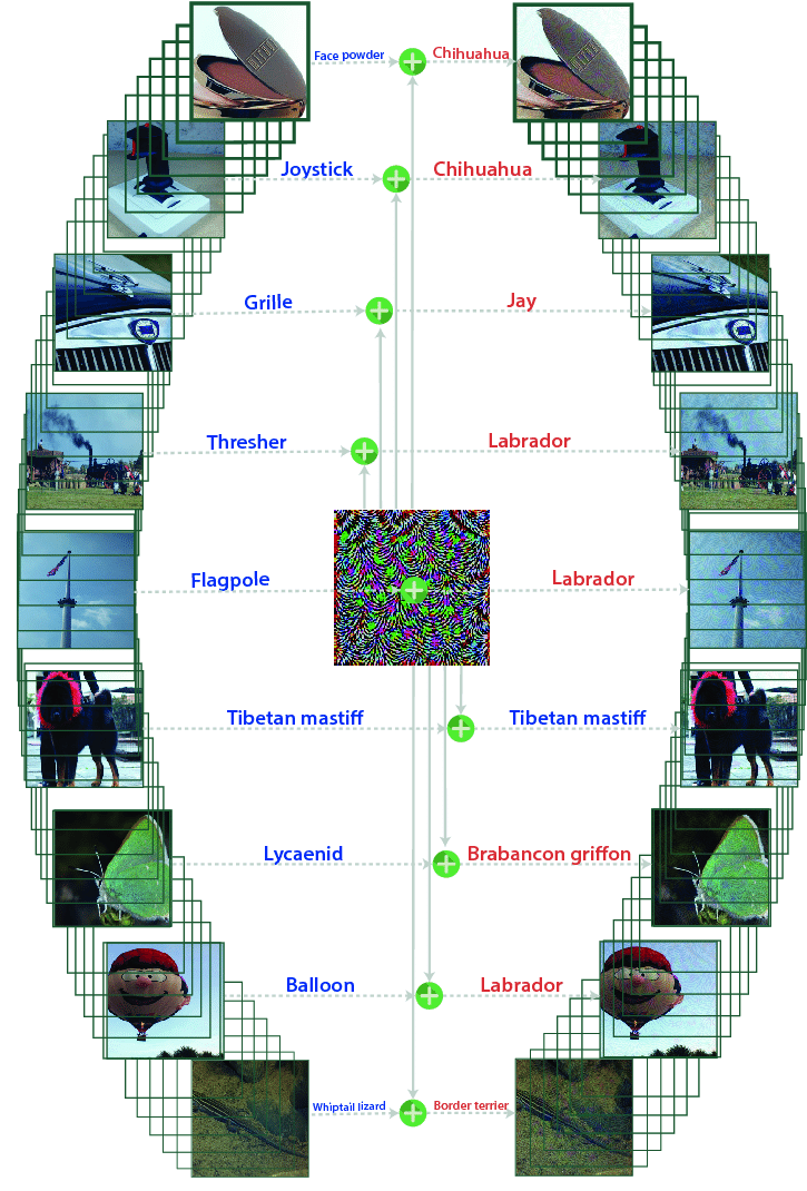
A single universal perturbation fools the model when applied to many images. The left column shows the original images, and the right column shows the images and classifications after applying the perturbation.
Image credit: Moosavi-Dezfooli et al.

Classification Boundaries

We can think of a neural network as a continuous function \(f: \mathbb{R}^d \to \mathbb{R}^\ell\), where \(d\) and \(\ell\) are the number of nodes in the input and output layers, respectively. Indeed, it is theoretically possible to write out a single mathematical expression for each of the output activations \(y_i\) in terms of the inputs \(x_1, \dots, x_d\). Although it would be extremely long, it would only involve addition, multiplication, and (if it’s using sigmoid) division and exponentiation. As a result, we can imagine the neural network as dividing \(\mathbb{R}^d\) into \(\ell\) classification regions, where region \(i\) corresponds to all inputs for which the model outputs the highest activation in node \(y_i\). Each of these regions is likely broken up into many disjoint components. Since it’s impossible to draw \(d\)-dimensional space where \(d\) is on the order of a million, in this post I’ll draw pictures with \(d = 2\).

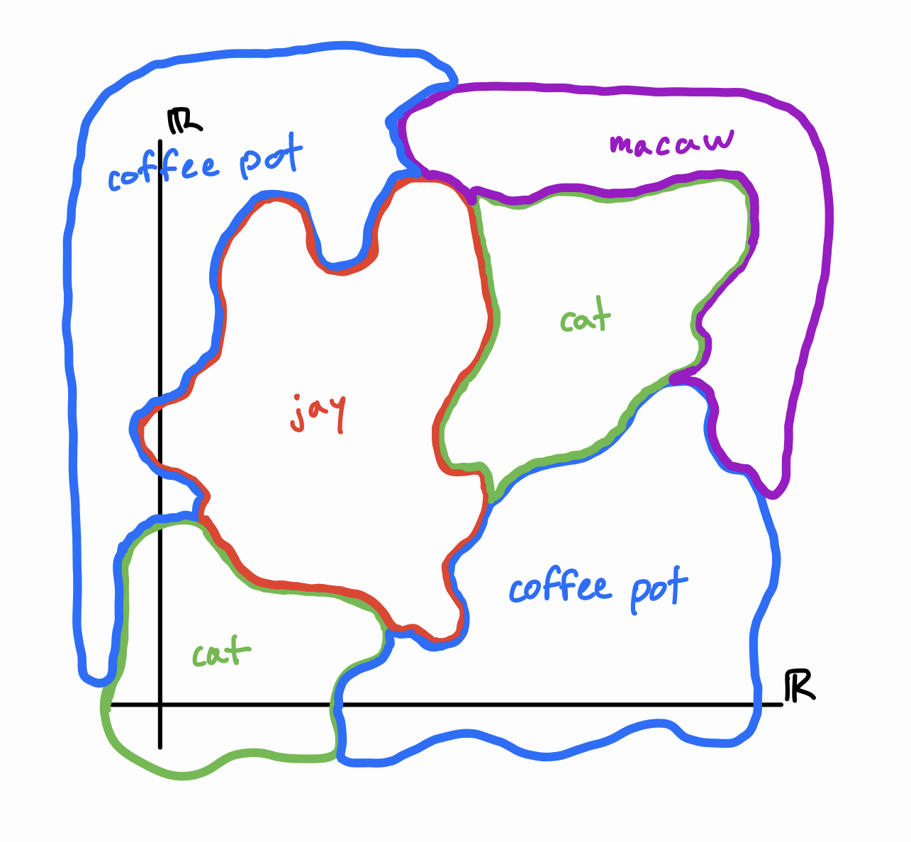
The hypothetical classification regions and boundaries of a neural net.

What can we say about the boundaries between regions? These correspond to inputs for which two distinct \(y_i\) and \(y_j\) are tied for the highest activation. If we’re using the sigmoid function (which is differentiable), we can prove that these boundaries are locally \(d-1\)-dimensional hypersurfaces. This means that if you zoom in close enough, the boundaries between regions should look nice and flat – they’re not going to have any weird fractal properties.

But this flatness is only guaranteed if we zoom in far enough. In practice, even though the function \(f\) is smooth, it can still look very un-smooth on human scales (in the same way that \(100 \sin (100 x)\) looks very un-smooth when you plug it into Desmos). This is what is going on with adversarial perturbations. A small change in \(x\) can lead to a large change in \(f\) because its linearity only becomes apparent for really really small changes in \(x\).³

Four Scenarios

I find it helpful to think of adversarial perturbations pictorially. What do adversarial perturbations tell us about the geometry of classification boundaries? Consider four hypothetical neural networks that have qualitatively different levels of robustness to perturbations. From most robust to least robust, these are (1) there are no adversarial perturbations, (2) there are adversarial perturbations (3) there are universal adversarial perturbations, and (4) all perturbations are adversarial. Each of these categories is strictly more robust than the next, in the sense that any type of perturbation that can fool model \(i\) can also fool model \(i+1\).

As you read through these scenarios, please keep in mind that the diagrams are meant as coarse 2D intuition builders, and nothing more. The actual classification boundaries in \(\mathbb{R}^d\) would look drastically different (if it were even possible to visualize \(d\) dimensions).

Category 1: There are no adversarial perturbations. In this ideal model, adversarial perturbations do not work. For almost all images in the real world distribution \(D\), there is no small \(\Delta\) we can add to it that will cause it to be misidentified. This means that a medium-sized ball centered around almost any point in \(D\) will still lie completely within the correct classification region. Written symbolically, this case roughly means \(\forall I \in D, \forall \Delta \in \mathcal{B}_ \epsilon, [f(I) = f(I + \Delta)]\) (where \(\mathcal{B}_ \epsilon\) is all points in \(\mathbb{R}^d\) with a small magnitude). This is what the classification boundaries would look like:

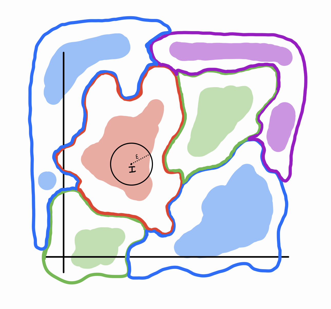
Notice the shaded sub-regions inside each classification region. These shaded sub-regions represent the test distribution \(D\), i.e. images that you would find in the real world. The color of a shaded region is the “ground truth”, i.e. the actual label of the image. When we make the assumption that our model is 100% accurate at classifying images in \(D\), this is equivalent to saying “purple shaded regions lie within purple boundaries, red shaded regions lie within red boundaries, etc.”

Almost all of \(\mathbb{R}^d\) corresponds to images of random-looking noise⁴ – only a tiny fraction of \(\mathbb{R}^d\) contains images that you would look at and say “yeah, that’s a cat/pillow/coffee pot”. Let’s call this set of images \(H\) for “human recognizable”. And only a small fraction of images in \(H\) are in \(D\) – images you would encounter in real life. For example, the unmodified picture of the coffee pot above is in \(D\), while the adversarially perturbed image of the coffee pot is not in \(D\) (although it is in \(H\)). After all, we are assuming that our neural net is 100% accurate on \(D\), so in order for a perturbation to fool the model, it has to knock the image outside of \(D\). Note that \(D \subset H \subset \mathbb{R}^d\), and any small perturbation of \(D\) should still lie in \(H\). You can think of \(H\) as the union of small neighborhoods surrounding points of \(D\).

We only care about the effect of adversarial perturbations on images in \(D\). So as long as the classification boundaries of \(f\) give a wide enough berth around the shaded regions, we can consider our model robust. An equivalent way of stating this is “our model is accurate on \(H\)”.

Category 2: There are adversarial perturbations. In this model, for most images \(I\) in the test distribution, there exists a small perturbation \(\Delta\) (chosen for a specific \(I\)) that fools the neural net. This case roughly translates to \(\forall I \in D, \exists \Delta \in \mathcal{B}_ \epsilon \,\text{s.t.}\, f(I) \neq f(I + \Delta)\).

Here’s one way that this could look:

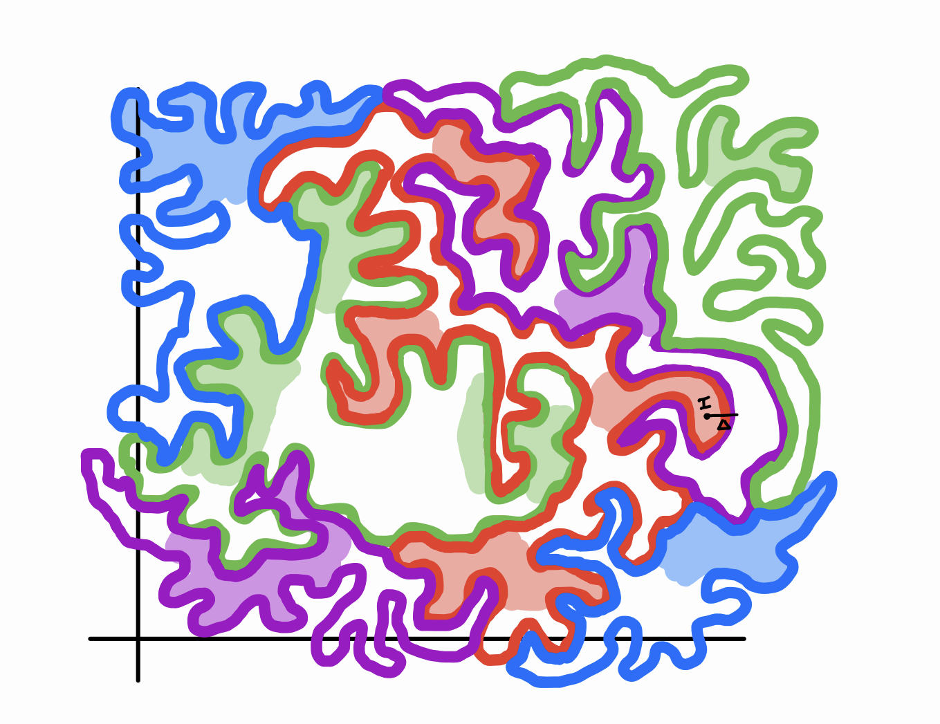
In this picture, the classification boundaries are very wrinkly, almost fractal-like. This gives them high surface area to volume ratios, which means that a randomly selected point inside one of these regions is likely to be close to a boundary. Thus, a small \(\Delta\) exists that will reach a different region when added to that point, fooling the model. A subtle (but important) property to notice is that different colored shaded regions are not close to each other: for any \(I, J \in D\), if \(f(I) \neq f(J)\), then \(\lvert I - J\rvert\) is big. This is because, assuming we have a finite set of disjoint classification options, there shouldn’t be any images in \(D\) that straddle the boundaries between categories. No real-life picture of a coffee pot looks very very similar to a real-life picture of a macaw. In fact, if this were not the case, then it would be hopeless to avoid adversarial perturbations because slightly modifying a coffee pot would actually result in a macaw.

Category 3: There are universal adversarial perturbations. This is the scenario that Moosavi-Dezfooli et al. showed to be true for the models they studied. The only difference between this and the previous scenario is the order of the quantifiers: \(\exists \Delta \in \mathcal{B}_ \epsilon \,\text{s.t.}\, \forall I \in D, f(I) \neq f(I + \Delta)\).

Here’s one way this could look:

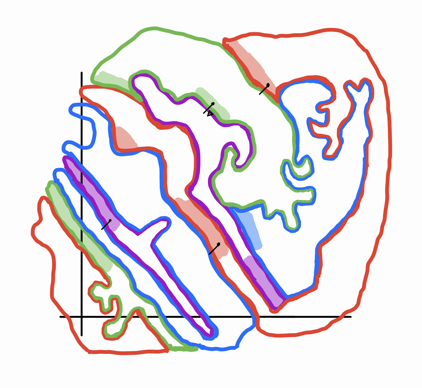
This image is a bit weirder. Like the previous category, it has skinny, almost fractal-like areas. But the important difference is where the shaded parts line up along the classification borders. Notice that there is a common direction in which all of \(D\) is “smeared”. This corresponds to a single direction for \(\Delta\) that successfully pushes all of \(D\) across a neighboring classification boundary. In other words, the tangents of classification boundaries near \(D\) are strongly correlated. This is in contrast with Category 2, in which the tangents of boundaries point in all different directions.

I was tempted to draw this category in a more simplified way: as a stack of thin pancakes, all oriented in the same direction. But in two dimensions, this gives the false impression that the classification regions all have to be the same shape. In reality, there can be lots of complexity and diversity to the shapes of the regions – it can just occur in the \(d-1\) other dimensions. In fact, as I have drawn, the regions are allowed to have thickness even in the direction of \(\Delta\), as long as \(D\) is always distributed on a specific side of each region.

Category 4: All perturbations are adversarial. This represents the worst-case scenario, in which the model completely flounders whenever you add a bit of noise to an image. This roughly means that \(\forall I \in D, \forall \Delta \in \mathcal{B}_ \epsilon, [f(I) \neq f(I + \Delta)]\). With this scenario comes the assumption that the topology of \(D\) is very disparate – more similar to a bunch of isolated points than a bunch of blobby regions:

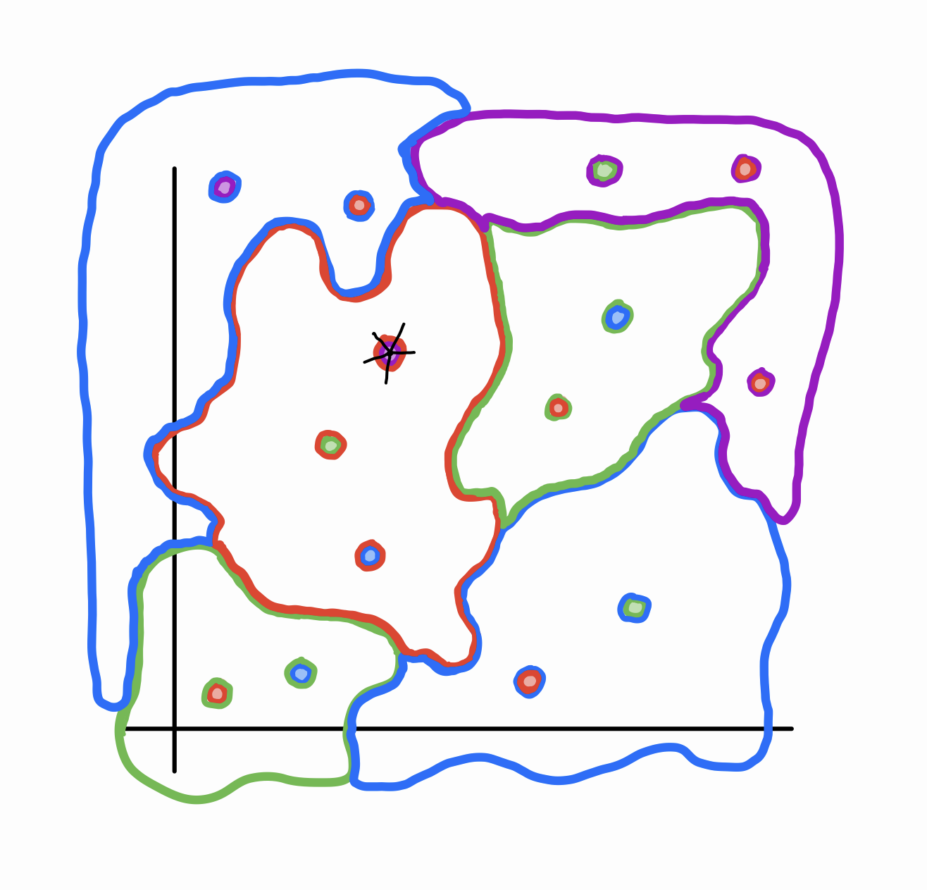
Notice that the shaded regions are in small bubbles contained in broader regions of a different class. I don’t expect that any image classification model would be bad enough to fall into this scenario.

Conclusion

In my opinion, the most important ideas brought up here are:

Thinking of a neural network as a continuous function from \(\mathbb{R}^d\) to \(\mathbb{R}^\ell\)
The distinction between \(D\), \(H\), and \(\mathbb{R}^d\)
Categorizing robustness to adversarial perturbations into these four types
The idea of the orientations of classification boundaries being “correlated”

Coming up with these four categories helped me understand the relationship between adversarial perturbations and the geometry of classification boundaries. I’m pleased with how each of the categories can be expressed by a logical formula, the only differences between them being the types and order of the quantifiers.

Finally, I want to mention that an obvious way that one could attempt to make a model more robust (i.e. bring it from Category \(i\) to Category \(i-1\)) would be to re-train it on perturbations of images in \(D\), either randomly or adversarially. The researchers tried this, with limited success – more details can be found in their paper. The paper also describes the algorithm they used to generate adversarial perturbations and a precise way to quantify how correlated the orientations of the classification boundaries are.

Thank you for reading! Please let me know if I have made any mistakes or if you disagree with parts of my analysis.

S. Moosavi-Dezfooli, A. Fawzi, O. Fawzi, and P. Frossard. Universal adversarial perturbations. In IEEE Conference on Computer Vision and Pattern Recognition (CVPR), 2017. https://arxiv.org/abs/1610.08401 ↩
In fact, they found perturbations that are doubly universal: they work on a large fraction of images on multiple different neural networks (VGG-F, CaffeNet, GoogLeNet, VGG-16, VGG-19, ResNet-152). ↩
The function \(f\) might be so sensitive that even the smallest change you can make to a digital image – modifying one color value by \(1\) out of \(256\) – could lead to large changes in \(f\). In other words, the straight-line path from \(I\) to \(I' = I + (0, \dots, 0, 1, 0, \dots, 0)\) could potentially cross multiple decision boundaries. ↩
Alternatively, you could interpret this as saying that the largest classification region by volume in \(\mathbb{R}^d\) is “TV static”. ↩