Thanks to Thomas Huck for suggesting the alternate method of finding $\mathbb{E}[T^2]$ mentioned in the conclusion.

The Problem

Consider the following problem about a random walk.

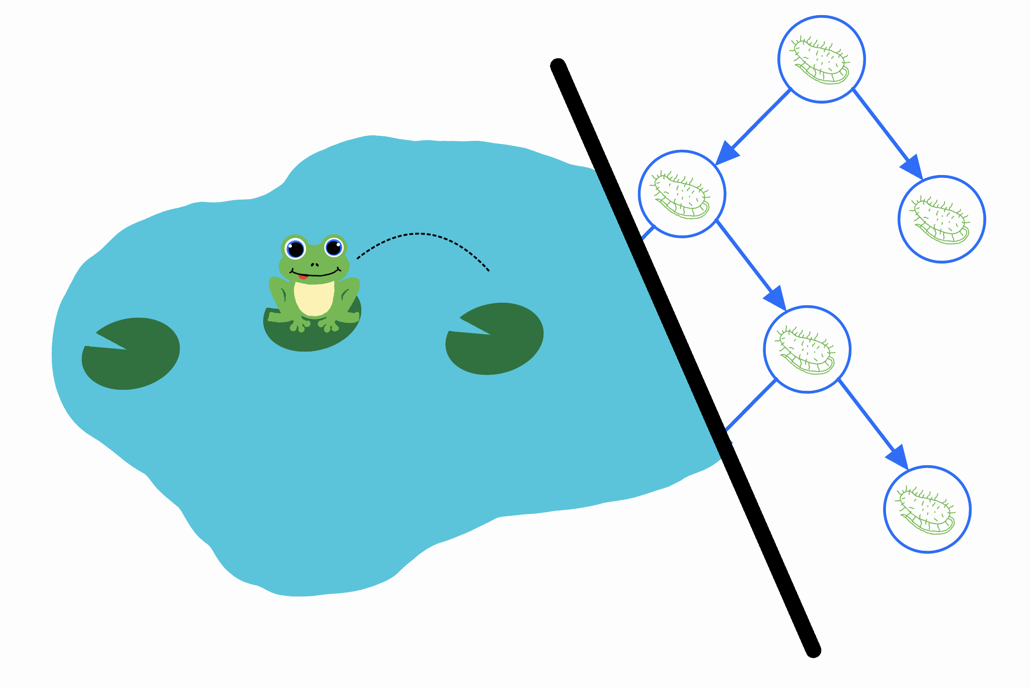
A frog starts at position $k$ on the number line. Every second, it takes a hop to the right with probability $p$ and left with probability $1-p$. Let $T$ be the number of hops the frog takes before it reaches $0$ for the first time (assume that $p < \tfrac{1}{2}$, so it always eventually reaches $0$). What is $\mathrm{Var}[T]$?

I’m sure there are many ways to solve this problem, but this post describes a solution that I’m particularly proud of. If you feel up for it, give it a try yourself before reading on!

First Steps

Let $T_{k \to (k-1)}$ be the number of hops the frog takes to reach $k-1$ if it starts at $k$. Let $T_{(k-1) \to (k-2)}$ be the number of hops it takes to reach $k-2$ if it starts at $k-1$. Defining $T_{(k-2) \to (k-3)}, \dots, T_{1 \to 0}$ in the same way, we can write

$$T = T_{k \to (k-1)} + T_{(k-1) \to (k-2)} + \dots + T_{1 \to 0}.$$

This is because we can break down the frog’s journey from $k$ to $0$ into a bunch of subtasks that must be completed in order: first it must reach $k-1$, then $k-2$, etc. But now we see that all of the random variables $T_{k \to (k-1)}, \dots, T_{1 \to 0}$ are independent and identically distributed. Why? Well, the frog’s jumps don’t depend on where it is on the number line or what previous jumps occurred, so the subtask of starting at $i$ and reaching $i-1$ should be the identical and independent for all $i$.

$T$ is the sum of $k$ i.i.d. random variables, so the variance of $T$ is $k$ times the variance of just one of them. Our job has been simplified to finding $\mathrm{Var}[T_{1\to 0}]$, which is equivalent to just solving the problem when $k = 1$ (in which $T = T_{1 \to 0}$). We’ll assume that $k=1$ from now on.

To find $\mathrm{Var}[T]$, it suffices to find $\mathbb{E}[T]$ and $\mathbb{E}[T^2]$ because $\mathrm{Var}[T] = \mathbb{E}[T^2] - \mathbb{E}[T]^2$. Finding $\mathbb{E}[T]$ can be done with a standard application of linearity of expectation. After the frog takes a single hop, there is a $1-p$ chance that it is at $0$ and a $p$ chance that it is at $2$. If it is at $0$ then it doesn’t need to take any more hops to reach $0$, but if it is at $2$, in expectation it requires $\mathbb{E}[T_{2 \to 1} + T_{1 \to 0}] = 2\mathbb{E}[T]$ more hops. So we write

\[\begin{align*} \mathbb{E}[T] &= 1 + p \cdot 2\mathbb{E}[T] \\ \mathbb{E}[T] &= \frac{1}{1-2p}. \end{align*}\]

Finding $\mathbb{E}[T^2]$, however, will require more work.

Representation as Bacteria

Imagine a colony of bacteria that starts as a single cell. Every second, one of the bacteria undergoes a change: with probability $p$ it splits into two new bacteria, and with probability $1-p$ it dies. This continues until there are no more bacteria alive.

We can track the population of the bacteria colony over time. In the above example, the population evolves as follows:

Time	$0$	$1$	$2$	$3$	$4$	$5$	$6$	$7$
Population	$1$	$2$	$3$	$2$	$1$	$2$	$1$	$0$

It’s not hard to see that the population of the colony follows the same random walk as the frog’s position: at every second, it either increases or decreases by $1$ with the same probability as the frog. Thus, the amount of time that the colony stays alive – or alternatively, the total number of bacteria that come into existence – has the same distribution as $T$. Now we’ve reduced our problem to figuring out: “what’s the expected square of the number of bacteria that come into existence”?

Math with Trees

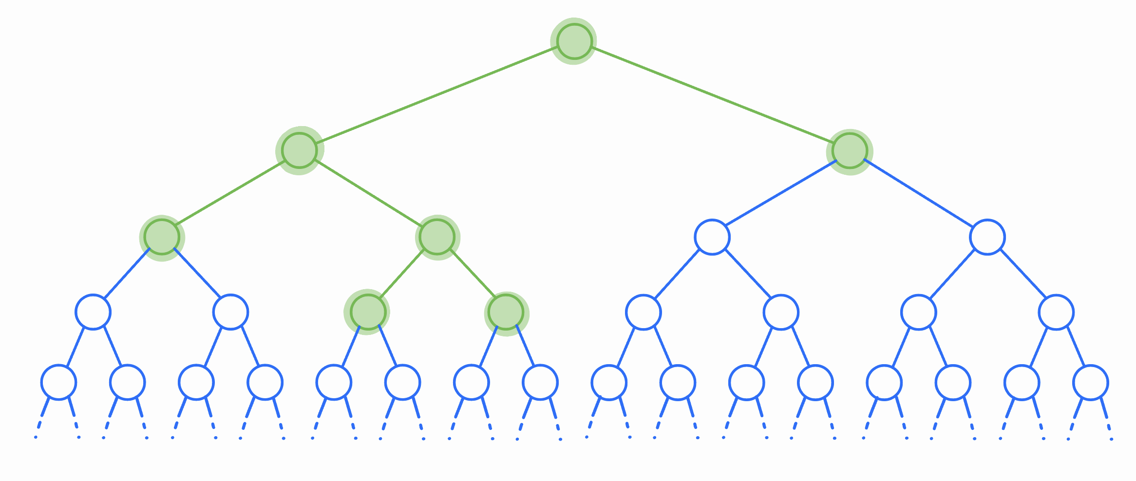
To answer this, we visualize all bacteria that could ever live as an infinite binary tree. Each node of the tree represents a potential bacteria, although in any given experiment only some of these bacteria will come into existence (the highlighted section of the tree represents the bacteria that lived in the above example).

Let’s solve for $\mathbb{E}\left[\binom{T}{2}\right]$: the expected number of unordered pairs of bacteria that ever exist. This is quadratic in $T$, so if we can do this we’ll be able to recover $\mathbb{E}[T^2]$. The expected number of pairs of bacteria that ever exist is the same as the sum, across all pairs of potential bacteria, of the probability that both bacteria in that pair exist. In other words, we’re writing $\binom{T}{2}$ as the sum of an infinite number of indicator random variables (one for each pair of potential bacteria), and then using linearity to write $\mathbb{E}\left[\binom{T}{2}\right]$ as the sum of the expectations of each of these indicators.

So how do we compute this infinite sum? To start, we can find the expected number of pairs of bacteria that come into existence and have the root node (the original cell) as their least-common ancestor. Recall that the LCA of two nodes $u$ and $v$ in a tree is the node of smallest depth on the unique path from $u$ to $v$. So in order for the LCA of $u$ and $v$ to be the root, we require either that

one of the nodes is in the left subtree of the root and the other is in the right subtree, or
one of the nodes has to be the root itself.

The number of pairs that come from the first case is $L \cdot R$, where $L$ and $R$ are the sizes of the left and right subtrees of the root, respectively. The number of pairs that come from the second case is $L + R$. Note that if the root never splits, then $L = R = 0$. Otherwise, with probability $p$, the root splits and we get $L, R \stackrel{iid.}{\sim} T$ (both $L$ and $R$ are independent and have the same distribution as $T$ itself). So we can write

\[\begin{align*} \mathbb{E}[\text{# of pairs with root LCA}] &= p \cdot (\mathbb{E}[LR] + \mathbb{E}[L + R])\\ &= p \cdot (\mathbb{E}[T]^2 + 2\mathbb{E}[T])\\ &= p \left(\frac{1}{(1-2p)^2} + \frac{2}{1-2p}\right)\\ &= \frac{p(3-4p)}{(1-2p)^2}. \end{align*}\]

This is great news, but we still need to account for all of the pairs that don’t have their LCA at the root. Fortunately, because of the self-similar structure of the tree, this is simple. For any node $u$ at depth $d$, the expected number of pairs that have their LCA at $u$ is simply the probability that $u$ comes into existence (which is $p^d$), times the expected number of pairs that have their LCA at the root (which is the formula we just found)! This is true because all bacteria are identical – once a bacteria is born, the distribution of the number of descendents it will have is the same no matter where it is in the tree.

Now we sum over all possible LCAs using a geometric series! Note that there are $2^d$ nodes at depth $d$, and every pair of nodes has a unique LCA (so we’re not over or under counting).

\[\begin{align*} \mathbb{E}\left[\binom{T}{2}\right] &= \sum_{\text{all nodes}\, u} p^{depth(u)} \cdot \frac{p(3-4p)}{(1-2p)^2} \\ &= \frac{p(3-4p)}{(1-2p)^2} \sum_{d=0}^{\infty} \; \sum_{u \,\text{at depth} \,d} p^{d} \\ &= \frac{p(3-4p)}{(1-2p)^2} \sum_{d=0}^{\infty} 2^dp^d \\ &= \frac{p(3-4p)}{(1-2p)^2} \cdot \frac{1}{1-2p} \\ &= \frac{p(3-4p)}{(1-2p)^3} \end{align*}\]

Putting it all together

With this result, we can recover $\mathbb{E}[T^2]$ by writing

\[\begin{align*} \binom{T}{2} &= \frac{T(T-1)}{2} \\ T^2 &= 2\binom{T}{2} + T \\ \mathbb{E}[T^2] &= 2\mathbb{E}\left[\binom{T}{2}\right] + \mathbb{E}[T] \\ &= 2\frac{p(3-4p)}{(1-2p)^3} + \frac{1}{1-2p} \\ &= \frac{-4p^2+2p+1}{(1-2p)^3}. \end{align*}\]

Finally, we get

\[\begin{align*} \mathrm{Var}[T] &= \mathbb{E}[T^2] - \mathbb{E}[T]^2 \\ &= \frac{-4p^2+2p+1}{(1-2p)^3} - \frac{1}{(1-2p)^2} \\ &= \frac{4p(1-p)}{(1-2p)^3}. \end{align*}\]

Thus, the answer to the original problem is

\[\begin{equation*}\boxed{\frac{4kp(1-p)}{(1-2p)^3}}\end{equation*}.\]

Conclusion

This solution technique is what the legendary Joe Blitzstein calls “reasoning by representation.” To answer a question about a distribution, we construct a random process that’s “isomorphic” to the first but has a more convenient structure for solving the problem at hand. In this case, we used the self-similarity of the tree structure to make counting pairs easy.

I’ll leave you with a slick alternate way to find the second moment of $T$ that manages to avoid an infinite sum. The total number of bacteria is expressible as $T = 1 + I(T' + T'')$, where $I \sim \mathrm{Bern}(p)$ and $T', T'' \stackrel{iid.}{\sim} T$ are two independent copies of $T$. Then

\[\begin{align*} T^2 &= \left(1 + I(T' + T'')\right)^2 \\ &= 1 + 2I(T' + T'') + I^2(T' + T'')^2 \\ \mathbb{E}[T^2] &= 1 + 2p(\mathbb{E}[T] + \mathbb{E}[T]) + p(2\mathbb{E}[T^2] + 2\mathbb{E}[T]^2) \\ (1-2p) \mathbb{E}[T^2] &= 1 + \frac{4p}{1-2p} + \frac{2p}{(1-2p)^2} \\ \mathbb{E}[T^2] &= \frac{-4p^2+2p+1}{(1-2p)^3}. \end{align*}\]

This method also makes it easy to find the higher moments of $T$ as well.