Recommended prerequisites:

expected value
linearity of expectation

Expected value (together with probability¹) is my favorite mathematical tool. One of the most appealing qualities of an expected value problem is that there are so many different ways of reaching the same answer.

I want to demonstrate this conceptual fluidity with a standard problem. Say you’re currently at position $3$ on the number line. Every second, you flip a fair coin to determine whether to take a step in the positive or negative direction. What is the probability that you reach position $10$ before position $0$? The answer is quite intuitive: $\frac{3}{10}$. In general, the probability a random walk reaches $+a$ before $-b$ is $\frac{b}{a+b}$. Here are four ways you can show this, each with its own advantages.

States from left to right

Let’s define $x_i$ to be the probability that you reach $i+1$ before you reach $0$ if you start at position $i$. This can occur in two ways: if your first move from position $i$ is to $i+1$ (this occurs with probability $\frac{1}{2}$), or if you first move to $i-1$, then you make it back to $i$ before hitting $0$, then you make it to $i+1$ before hitting $0$ (this occurs with probability $\frac{1}{2}x_{i-1}x_i$). In total, we get the recurrence $x_i = \frac{1}{2} + \frac{1}{2}x_{i-1}x_i$, which simplifies to $x_i = \frac{1}{2-x_{i-1}}$.

Our base case is $x_0 = 0$. Applying our recurrence, we get $x_1 = \frac{1}{2}$, $x_2 = \frac{2}{3}$, $x_3 = \frac{3}{4}$, and so on. We can prove that this pattern holds inductively: if $x_i = \frac{i}{i+1}$ then $x_{i+1} = \frac{1}{2 - \frac{i}{i+1}} = \frac{i+1}{i+2}$.

The original problem asks for the probability we reach $10$ before we reach $0$ when we start at $3$. For this to happen, we first need to reach $4$, then we need to reach $5$, and so on until we get to $10$ (avoiding $0$ at each step). This is exactly equal to the product $x_3x_4\dots x_9 = \frac{3}{4}\frac{4}{5}\cdots\frac{9}{10}$, which conveniently telescopes into our final answer: $\frac{3}{10}$.

Pros to this approach. This was the method my brother used when I presented this problem to him. My brother is primarily a competitive programmer, so building up states like this was the most natural solution to him. In the world of competitive programming, explicit recurrences are incredibly useful in a technique called dynamic programming. In particular, we seek one-sided recurrences (i.e. $x_i$ only depends on $x_{i-1}$, not $x_{i+1}$) so that values can be easily computed by iterating through a single index. The best label for this approach might be computationally-focused – it easily translates to an efficient algorithm.

Cons to this approach. This is the most algebraically-intensive approach described here, and perhaps the only one that you would need to pull out scratch paper for. As with any algebra-based approach, some amount of intuition and elegance is sacrificed in the complexity of the formulas. You can follow each individual step, but once you reach the end it’s hard to look back and say, “ah yes, now I see why it must have been $\frac{3}{10}$ all along.”

States, a global approach

This time we again use states, but we use a slightly different definition and get a different recurrence. Let $z_i$ represent the probability that you reach $10$ before you reach $0$ if you start at $i$. Our final answer will be $z_3$. For $1 \leq i \leq 9$, we know that $z_i = \frac{z_{i-1} + z_{i+1}}{2}$ because there is an equal chance of going to states $i-1$ or $i+1$ from $i$. In other words, each $z_i$ is the average of its two neighbors. At the endpoints, we have $z_0 = 0$ and $z_{10} = 1$.

What types of sequences set each element at the average of its neighbors? Straight lines! Or more specifically, arithmetic sequences. We can see that an arithmetic sequence is the only possible solution: whatever the difference between $z_1$ and $z_0$ is, this must be the same as the difference between $z_2$ and $z_1$, and the difference between $z_3$ and $z_2$, and so on. Thus, the value of $z_i$ is directly proportional to $i$. We get our final answer of $z_3 = \frac{3}{10}$.

Pros. This approach uses states more elegantly than the first method. We could have solved up a big linear system of equations once the recurrences were formed, but instead, we took a step back and ask what shape of solutions we were expecting. This allowed us to avoid doing algebra and gives us a much better intuition of where the answer comes from: your probability varies linearly on a local scale, so it must also vary linearly on a global scale.

Cons. We were lucky that the state recurrence was so simple. In different problems the recurrence can get more complex, so a global perspective does not always help. Sometimes, algebra is inevitable.

Circular symmetry

We start with a related problem. There are $11$ equally spaced points around a circle. A a wolf standing at one of these points, and sheep standing at the rest. Every second, the wolf travels one step clockwise or counterclockwise (with equal chance), eating any sheep along the way. The wolf will continue until it has eaten all of the sheep. What is the probability that $A$ is the last sheep the wolf eats?

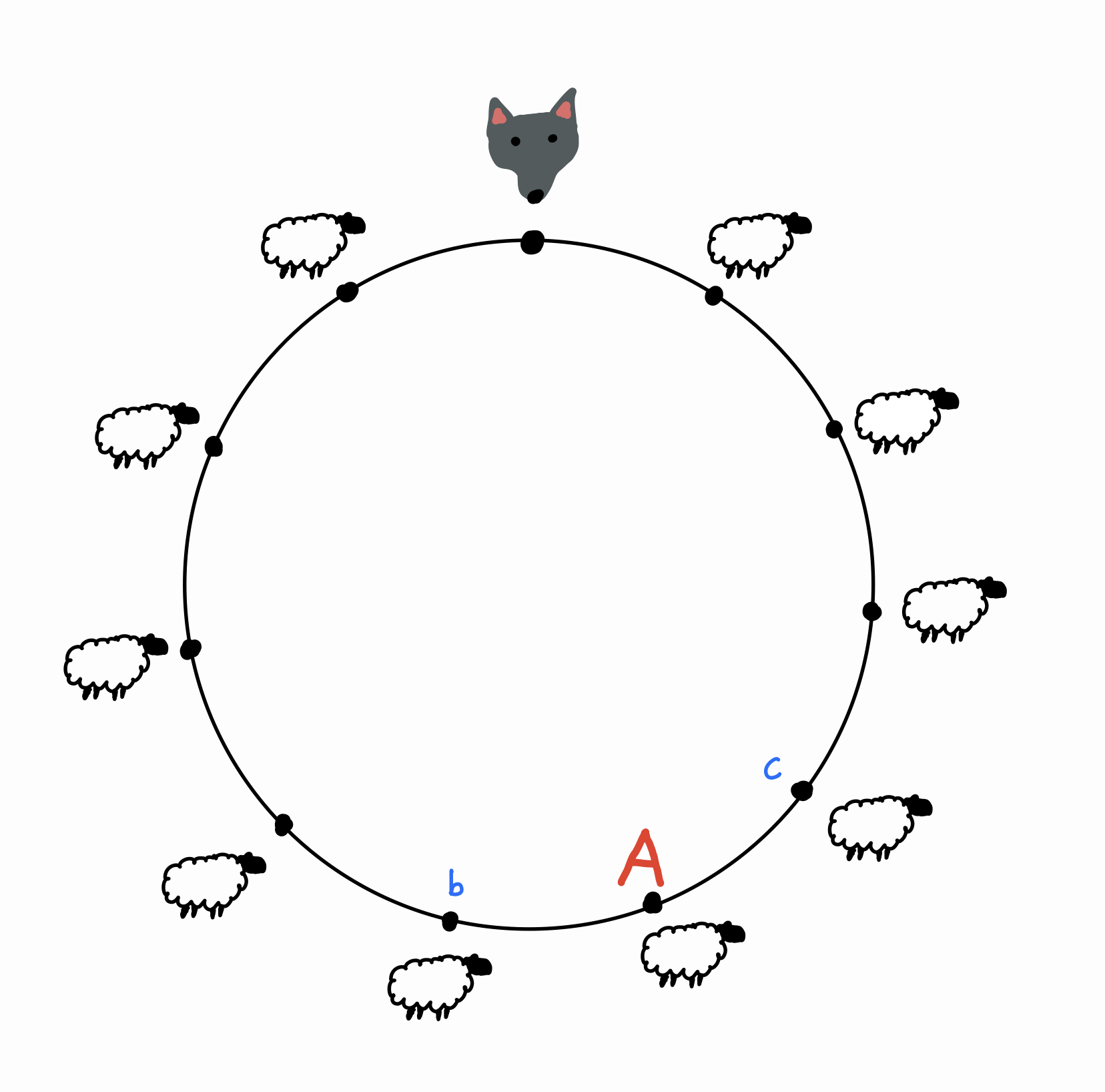
Here’s a slick way to answer this question. Without loss of generality, say that the wolf visits point $b$ before point $c$ (the other case is handled symmetrically). Let this be the first time that the wolf is next to $A$. Then in order for $A$ to be the last point visited, the wolf must make it all the way around the circle clockwise to point $c$ before it reaches $A$. In other words, the probability that $A$ is the last sheep eaten is the same as the probability that the wolf reaches a point $9$ positions clockwise before a point $1$ position counterclockwise. Let’s call this probability $x$.

But now realize that this chain of logic works for any sheep! The probability that any given sheep $S$ is last to be eaten is exactly $x$: there must be some first time that the wolf is next to $S$, then the wolf must make it all the way around to eat the other neighbor of $S$ before it eats $S$. So each sheep has the same chance of being the last survivor, and since there are $10$ sheep, this must be a probability of $\frac{1}{10}$.

This is a neat solution, but how does it help us with our original problem? Let’s label the points like this:

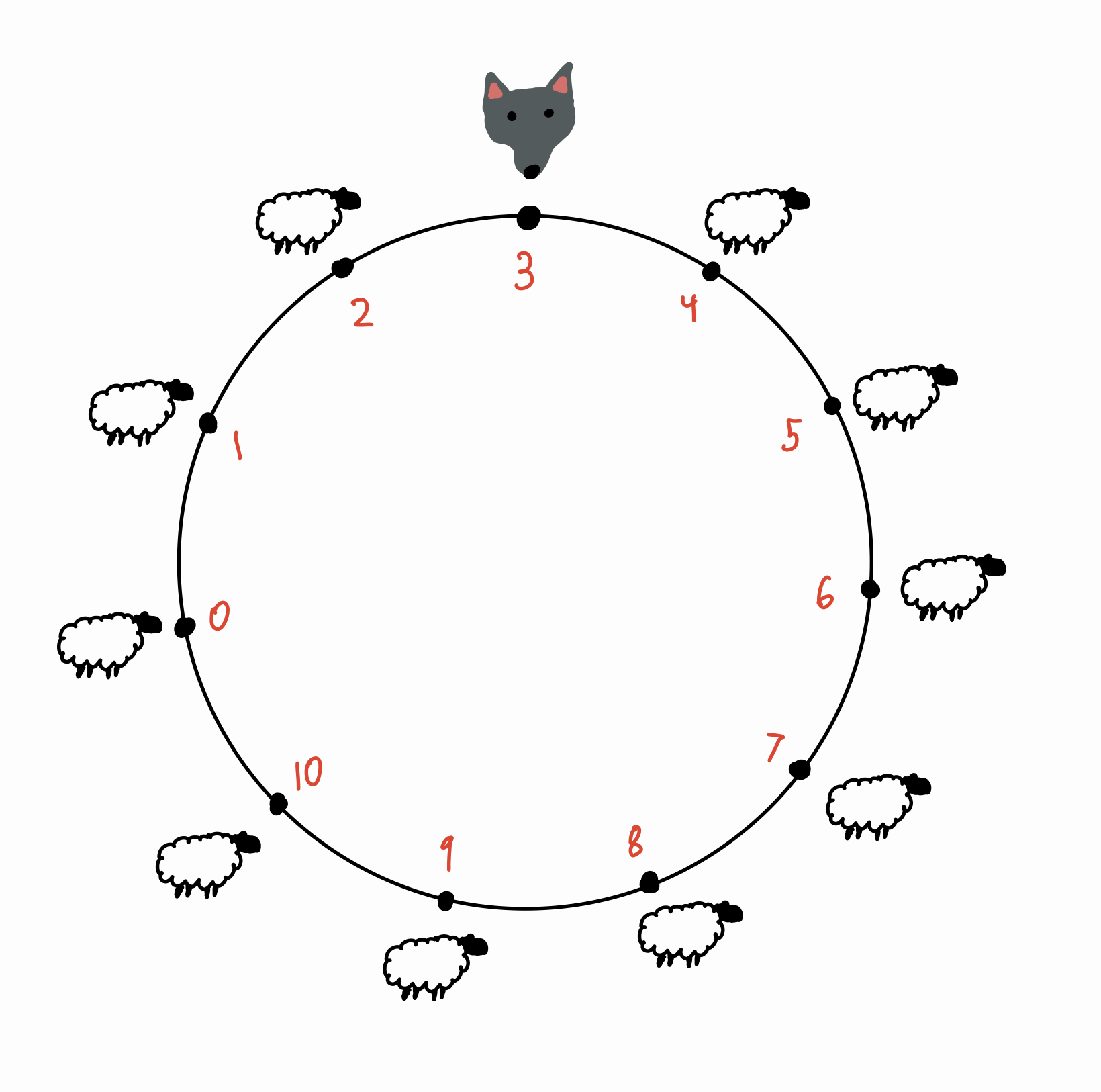
Now our problem is equivalent to finding the probability that the wolf eats sheep $10$ before sheep $0$. Here comes the key observation. If the last sheep it eats is $0$, $1$, or $2$, then the wolf must have eaten sheep $10$ before sheep $0$. Otherwise, if the last sheep it eats is one of $4, 5, \dots, 10$, then the wolf must have eaten $0$ before $10$.² This is great news because we already know each sheep has a $\frac{1}{10}$ probability of being eaten last! Thus, our final answer is $\frac{3}{10}$.

Pros. I think this is the “coolest” method listed here because of how it leverages symmetry around a circle. For another example of this, see Eric Neyman’s proof of Laplace’s Rule of Succession.

Cons. This is the longest (and possibly, most complex) method listed here. And despite the elegance of the approach, it is hard to see how it could be motivated. I will note, however, that this was the first method I came up with. This is probably only because I had recently been thinking about the wolf and sheep problem (it came up on a friend’s STAT 110 problem set).

A fair game

You are playing a betting game with your friend. You start with $\$3$, and your friend starts with $\$7$. Every turn, you flip a coin. If heads, you take a dollar from your friend, and if tails, your friend takes a dollar from you. You keep playing until someone runs out of money. It should be clear that this setup is identical to the original problem. We are interested in the probability that you win all $\$10$.

Notice that this game is fair, meaning that at every step of the game your wealth changes by an expected value of $0$. Thus, the expected value of your money at the start of the game is the same as the expected value of your money after the game! Since your money at the start of the game is $\$3$, there must be a $30\%$ chance that you end up winning the $\$10$.³

Pros. This is the simplest and (in my opinion) the most elegant of all of the methods listed here. It highlights the fluidity between probability and expected value. We took the probability of a random walk and reframed it as a game with money, and then as soon as we said the words “expected value” we found the answer staring us in the face.

Cons. I saved this method for last because it was actually the last one I thought of! Sometimes a solution is so natural that it takes a bit of thinking before you even consider it – and in that time you will have already thought of something else.

The concepts of probability and expected value are very strongly related. You often use one to think about the other, so I tend to group them together as a single concept. ↩
It is fairly easy to convince yourself of this fact by tracing your finger along possible wolf routes. But to be more rigorous, you can observe that “$0$ is visited before $10$” implies “$1$ is visited before $10$”, which implies “$2$ is visited before $10$”. So if you assume the negation of one of these statements (which is what you get with “$0$, $1$, or $2$ is the last sheep visited”), a chain of contrapositives should result in “$10$ is visited before $0$”. The other case works similarly. ↩
This type of fair game is also called a martingale, which comes with a bunch of theorems that we are implicitly invoking in this solution. ↩