Polya's Urn with Bayesian Updating
Polya’s Urn
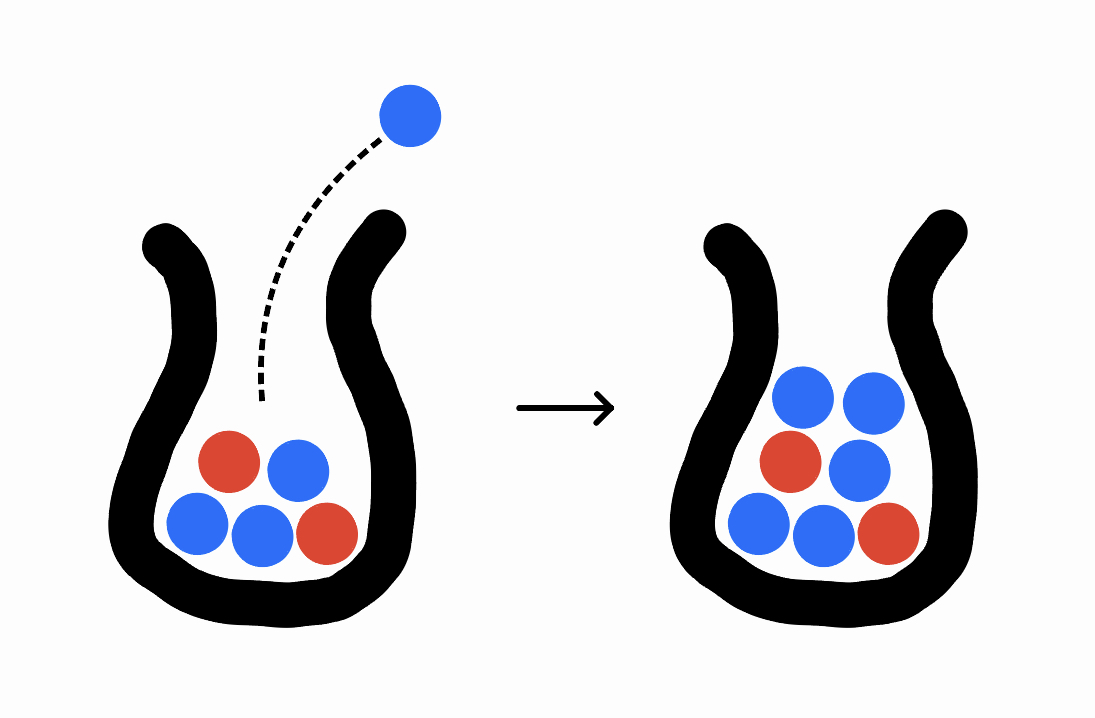
Polya has an urn that starts out with one blue ball and one red ball. Every day, he draws a random ball from the urn, duplicates it, then returns both copies to the urn. He keeps doing this until there are a very large number of balls in the urn. Finally, he looks inside and computes the proportion \(X\) of the balls that are blue. What is the distribution of \(X\)?
We can easily see that the expectation of \(X\) must be \(\tfrac 12\) by symmetry (the distribution of \(X\) must be the same as the distribution of \(1 - X\)). But is it clustered towards the center? Always either 0 or 1? If you don’t already know, take a moment to guess before continuing.
It turns out that \(X\) is uniformly distributed from \(0\) to \(1\). (Formally, if you let \(X_n\) be the ratio after \(n\) days, then \(X_n\) converges in distribution to \(\mathrm{Unif}(0, 1)\).) One way to see this is to directly calculate the probability that you have \(b\) blue balls after \(n\) days; if you expand out the “choose” formula and cancel things out you’ll see that it’s always exactly \(\frac{1}{n+1}\) no matter what \(b\) is – the ratio is distributed uniformly over all possibilities.
Here, I want to present an alternative, more intuitive way of seeing why \(X\) must have a uniform distribution. We’ll only need one tool to prove this: Laplace’s Rule of Succession.
Laplace’s Rule
A coin-making machine creates weighted coins that have head-probabilities \(p\) uniformly distributed from \(0\) to \(1\). Say I hand you a coin from this machine and you flip it \(n\) times, observing \(h\) heads and \(t = n-h\) tails (the order won’t matter). Conditioned on these observations, what’s the probability that your next flip is a head?
The answer is \(\frac{h+1}{h+t+2}\). This is a wonderful fact known as Laplace’s Rule of Succession, which Eric Neyman gives an elegant proof of here. If you haven’t seen the proof before (it centers around a symmetry argument on a circle), I highly recommend taking a look.
Two Identical Processes
Now we can prove our original claim. Let \(x_i\) be the color of the \(i\)-th ball we end up drawing (represented as a \(0\) or a \(1\)). Polya’s process defines some distribution over infinite binary strings \(x_1x_2x_3\!\dots\). If we let \(r(x_1x_2x_3\!\dots)\) be the “limiting ratio”
\[\lim_{n\to\infty} \frac{\sum_{i=1}^n x_i}{n},\]then we’re interested in showing that the distribution of \(r\) is uniform (it will later become clear that \(r\) must exist almost surely).
Next, consider a second setup. I give you a coin with head-probability \(p\) distributed uniformly. You flip the coin and write down the result as \(y_1\) (1 if heads, a 0 if tails). Then you flip it again and record it as \(y_2\), and so on. This new process once again results in a distribution over infinite binary strings \(y_1y_2y_3\!\dots\).
It turns out that these two distributions are identical! To show this, we’ll show that when generating the string digit-by-digit, both processes always give us the same probability of the next digit being \(1\). Laplace’s rule tells us that under the second (coin flipping) process, the probability that the next flip is heads is just \(\frac{h+1}{h+t+2}\). This can be written as
\[y_{n+1} = 1 \qquad \text{w.p.} \qquad \frac{1 + \sum_{i=1}^n y_i}{2 + \sum_{i=1}^n y_i + \sum_{i=1}^n (1-y_i)} = \frac{1 + \sum_{i=1}^n y_i}{2 + n}.\]What about the first process? Well, given that the first \(n\) balls we’ve drawn so far have been \(x_1, \dots, x_n\), the probability that the next ball we draw is blue is just the number of blues in the urn divided by the total number of balls. There is one blue ball in the urn for every previous blue ball we’ve drawn (plus one for the original blue ball), and there are \(n + 2\) total balls. Thus,
\[x_{n+1} = 1 \quad \text{w.p.} \quad \frac{1 + \sum_{i=1}^n x_i}{2 + n}.\]We conclude that the two processes induce the same distribution over binary strings. Now we just want to know the distribution of \(r(y_1y_2y_3\dots)\). By the law of large numbers, as you flip a coin more and more times the ratio of heads converges to the underlying head-probability \(p\) of the coin. Since the distribution of \(p\) is uniform by assumption, we’re done!1
Other Starting Conditions
What if instead of starting with only one blue and one red, Polya had started with \(b\) blues and \(r\) reds? Our new Bayesian understanding of this process immediately tells us that the distribution of \(X\) must converge to the posterior distribution of \(p\) after seeing \(b-1\) heads and \(r-1\) tails – this is just \(\mathrm{Beta}(b, r)\).
And if he started with \(b\) blues, \(r\) reds, \(y\) yellows, \(g\) greens… it’s now the Dirichlet distribution!
-
I’ve swept under the rug some probability-theoretic details to this proof. A fully rigorous proof would have to demonstrate that, not only does any given string \(y_1y_2y_3\dots\) converge to its limiting ratio \(p\), but that the distribution of ratios of longer and longer prefixes converges to the distribution of \(p\). The quantifiers here are out of order. ↩