I would like to thank Alex Cai for the wonderful discussion that inspired this blog post.

Warning: mild blasphemy. Don’t take the conclusions of this post too seriously because I am not confident about many of these ideas.

* * *

Skeptical Scenarios

Attaining true knowledge is hard. As far as I know, I could be a brain in a vat with my nerve endings connected to wires that are simulating physical experiences. Gravity could reverse directions every 13.8 billion years, the first time being tomorrow. Or, our entire universe could be a simulation running on some alien supercomputer.

These are all skeptical scenarios: potentially absurd descriptions of “the way the universe is” that are consistent with all of my observations. Skeptical scenarios are impossible to rule out. No matter how hard I think about it, I will never be 100% confident that I am not a brain in a vat. Any scenario that doesn’t result in a logical contradiction with my observations has a nonzero possibility of being true.

While we can never rule out a skeptical scenario, we can certainly talk about how probable certain scenarios are over others. This may be good enough for all intents and purposes. For example, consider the following two skeptical scenarios:

The un-skeptical scenario (aka the Default View):

The universe is, more or less, what modern scientists believe it to be. Matter and energy behave according to fixed physical laws that we understand well (ignoring weird quantum interactions). There is nothing else to it besides these laws – no deities, no simulation, no brains in vats.

The Beatriz Scenario:

The entire universe was created by an omnipotent three-eyed goddess named Beatriz who has slimy green skin and 17 horns on her head. After we die, Beatriz sends our souls to live forever in an infinite field containing nothing but $42^n+9$ red dandelions, where $n$ is the number of Cheetos you ate during your life. Also, Beatriz’s favorite number is $758942678329405289$.

Both of these scenarios are possible – we don’t have any proof that Beatriz doesn’t exist. However, I find the Default View to be much more likely than the Beatriz Scenario, and I’m guessing that you do too. In fact, I don’t even consider the latter when making my daily decisions – I would never increase my Cheeto intake for the possibility of extra dandelions just in case the Beatriz Scenario happens to be true. The reason that I have a strong bias towards the Default View is its simplicity. It assumes nothing about the universe besides what scientists have already observed to hold. And although empirical scientific data doesn’t prove anything about the universe (for all we know, gravity could reverse directions tomorrow), it feels extremely natural that the simple physical laws we’ve formulated to match the data should end up being true. The Beatriz Scenario, on the other hand, is very complex because it makes many arbitrary choices. Thus, it feels less likely to be true.

We can formalize this notion of “simpler universes are more likely to be true” with two ideas: Bayesian probability and Kolmogorov complexity.

Bayesian Probability

We’re going to use the Bayesian view¹ of probability in this blog post. When applying Bayesian probability, we first need a “prior”: a probability distribution of “the way the universe is” that we would have before making any observations. Then, once we make observations about our universe, we “update our prior” by conditioning it our observations. This updated prior constitutes our final prediction about the universe we live in.

For example, imagine generating a Minecraft world from a random seed. Before the world renders, you have some prior about the way the world will be: maybe you think there’s a 50% chance you spawn in a forest biome, a 30% chance you spawn in the desert, and a 20% chance you spawn in the mountains. Then, once the world renders, you make some observations about your surroundings: perhaps you see lots of trees. This lets you update your prior with your new knowledge. Since a desert would never contain trees, the probability you assign to being in a desert drops to 0%. Meanwhile, the probability you assign to being in a forest goes up because forest worlds have lots of trees. The probability you assign to being in the mountains may go up or down depending on how likely you think it is to see trees in the mountains. As you explore your new world and make more observations, your internal probabilities keep updating. Bayes’ rule gives an explicit formula for these probability updates.

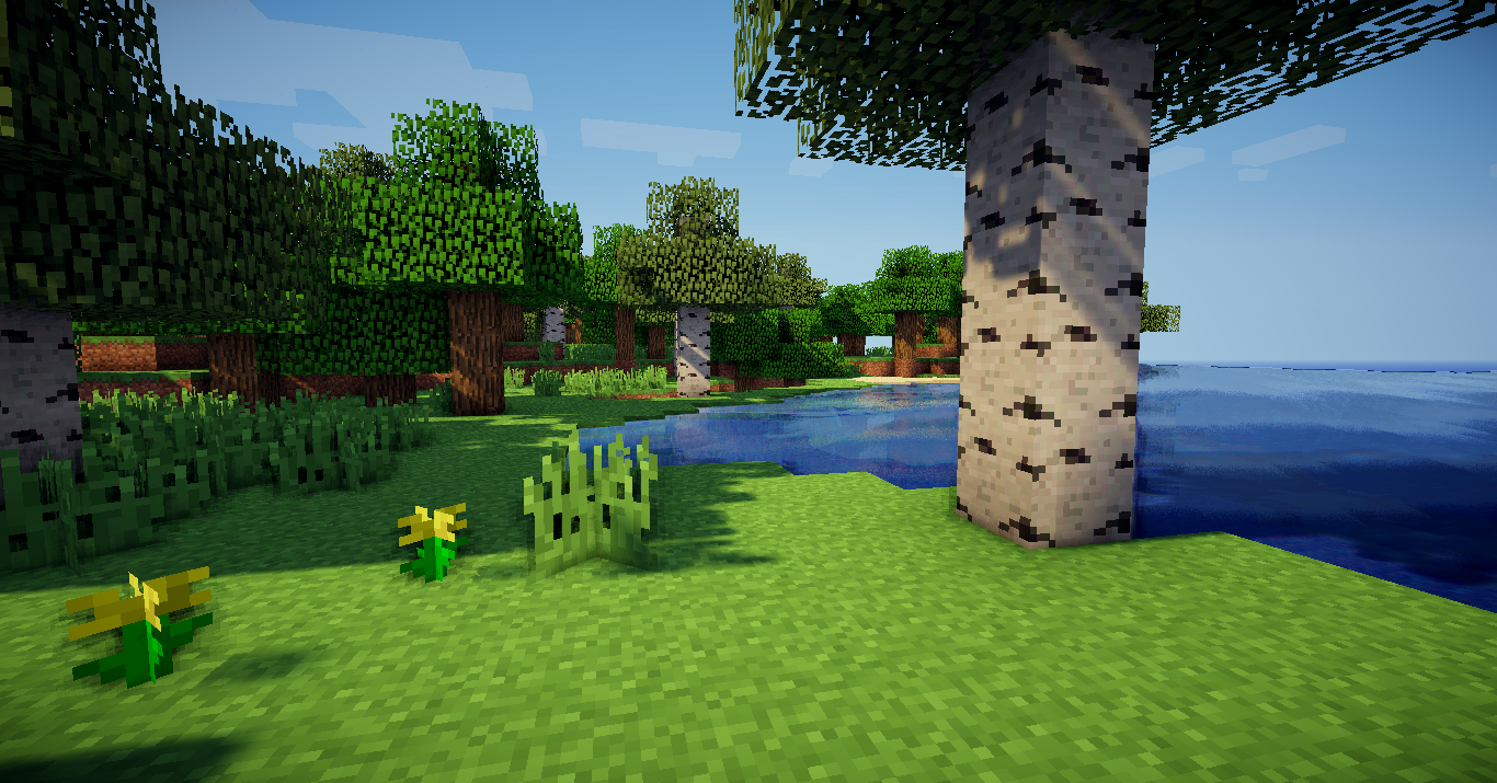
Feeling a warm pixelated breeze, you slowly open your eyes to a nascent Minecraft world. You see trees. Time to update those priors.

We can use the same idea to reason about our own universe. The tricky part is to come up with a good prior. Imagine yourself as an unborn fetus, still floating around in amniotic fluid. Lacking eyes and ears, you have yet to receive any information about the universe you are destined to enter. A priori, what would you expect the universe to be like? Would you believe a universe with multiple conscious beings to be more or less likely than a universe with only one? Would the existence of God be surprising or expected? Would the Default View seem more or less likely than the Beatriz Scenario?

The answer to this question, if it exists, is certainly not obvious. As alluded to in the first section, in this post we’ll use a prior based on simplicity. This stems from Occam’s Razor: the simpler the explanation, the more likely it is. We will create a prior probability distribution that assigns more weight to universes that are simpler to describe.

Kolmogorov Complexity

To formalize this idea of the “simplicity” of a universe, we turn to Kolmogorov Complexity. The Kolmogorov Complexity (KC) of an object is the length of the shortest computer program that produces the object as output. For example, the KC of the string afqb5CAfXzh#Nz5rT3S@f$JR59Jxt@ is much higher than the KC of aaaaaaaaaaaaaaaaaaaaaaaaaaaaab. Even though the two strings are the same length, the second one is computable by the short program print("a"*29+"b") in Python, while you can’t do much better than print("afqb5CAfXzh#Nz5rT3S@f$JR59Jxt@") for the first one.

The syntax of the programming language we’re working in doesn’t really matter – as long as we have a Turing-complete language like Python or C++, the Kolmogorov Complexity of any object will be the same up to a constant. You can think of KC as measuring the total amount of information stored in an object: its inability to be compressed. A string may be extremely long, but if its structure is very predictable, it will have a low KC because it is not very information-dense. There is a strong connection between KC and information-theoretic entropy.

So what is the KC of our universe? Assuming the Default View, we could hard-code the position of every fundamental particle at every point in time into our program. Think of this as taking a high-resolution video of the universe. This would result in an extremely long program. On the other hand, we could save a lot of space by specifying the laws of physics, along with certain initial conditions. The state of the universe over time could then be deterministically computed from the initial conditions and physical laws. This would result in a much shorter computer program.²

Now we can define a prior over universes! We want to have a distribution in which universes of lower KC are more probable. Let’s say that the prior probability that our universe has a KC of $n$ bits is $2^{-n}$ (this sums to $1$ over all $n$), and that all universes of a given KC are equally likely. Since there are at most $2^n$ potential universes with a KC equal to $n$ (there are only $2^{n}$ total programs of length $n$), we get that the prior probability of any given universe of KC $n$ is at least $2^{-2n}$. Let’s assume that this probability is exactly $2^{-2n}$ for the sake of simplicity.³

Of course, the choice of $2^{-n}$ was arbitrary; we could easily have used any other function $f(n)$ such that $\sum_{n=1}^{\infty} f(n) = 1$. For most reasonable functions $f$ the following conclusions will still hold, so I will use $2^{-n}$ to keep the calculations easy.

Remember that we still need to update our prior based on our observations. A universe tessellated with nothing but vegan hot dogs has a low KC, but it has $0$ probability of being true because it does not match what we observe. However, given two universes that both conform to our observations (such as the Default View and the Beatriz Scenario), we can discuss their relative probabilities by comparing their priors. The Beatriz Scenario probably has a higher KC than the Default View – after all, a program outputting the Beatriz Scenario has to output our physical universe in addition to the information about Beatriz – so it is less probable.

In fact, since our prior ranges over descriptions of entire universes (there’s no notion of chance), we can say that, given any hypothetical universe, the probability of making the observations that we did is discrete: either $0$ or $1$. This simplifies things under Bayes’ Rule⁴ by letting us say that the relative probabilities of two skeptical scenarios given our observations are the same as they were in the prior distribution.

A universe tessellated with nothing but vegan hot dogs.

A Lower Bound

We can finally state the main conclusion of this blog post.

Assuming such a prior, any skeptical scenario you can think of, no matter how contrived or absurd, must be at least $2^{-400}$ as likely as the Default View.

How can this be possible? After all, can’t there be skeptical scenarios of arbitrarily large KC, which gives them arbitrarily low probabilities relative to the Default View?

The answer is the presence of the phrase “you can think of”. The fact that you thought of a skeptical scenario gives an upper bound on its Kolmogorov Complexity.

Lemma: The KC of any skeptical scenario you can think of is at most the KC of the Default View, plus 200 bits.

Proof of Lemma: Consider any skeptical scenario $S$ that you think of, for example the Beatriz Scenario. There exists the following program that outputs $S$. First, start with the code of the shortest program that outputs the Default View (say this requires $n$ bits). Modify the code so that, instead of outputting the Default View, it computes and stores the entire history of the Default-View-universe in an intermediate variable. Then, hard-code in a new variable that “points” to yourself at a time in which you are thinking of $S$. This variable must specify the exact second in which you were thinking about $S$, along with some information that distinguishes you apart from all other thinking beings in the universe at that time.

How many bits of information does this require? Well, the time stamp can be encoded in a number approximately equal to the number of seconds that have passed since the start of the universe, which is around $13 \times 10^9 \cdot 365 \cdot 24 \cdot 3600 \approx 4 \times 10^{17}$. This requires $60$ bits of information. Given this point in time, to point to you, the human being specifically, we can first point to our Sun, then point to you as a thinking creature in the Sun’s planetary system. Scientists believe there could be around $10^{24}$ stars in the universe, so we would need $80$ bits of information to single out the Sun. There are only $\approx 10^{10}$ humans in our solar system, so we would require another $35$ bits of information to point to you. Altogether, this pointer would require $60 + 80 + 35 = 175$ bits of information. We can round up to $200$ to account for having very sloppy estimates.

Now that we have a pointer consisting of $200$ bits, we can simply point to $S$ in your brain at the given time and have the program output whatever skeptical scenario you’re thinking of, whether it be the Beatriz Scenario or something much more contrived. This program has a length no more than $n + 200$. Thus, $KC(S) \leq KC(\text{Default-View}) + 200$. $\blacksquare$

The final result follows easily from the Lemma. Since both the Default View and $S$ conform with our observations, their relative probabilities are the same as their relative probabilities in the prior probability distribution, which must be at most $2^{-2 \cdot 200} = 2^{-400}$.

The Consequences

I’ll be the first to admit that $2^{-400}$ is an extremely tiny number. This means that at a first glance, our lower bound is extremely weak. But when you think about it, $2^{-400}$ is quite large compared to how absurdly contrived I could make a skeptical scenario. For example, I could modify Beatriz’s favorite number to be the gargantuan integer that I get by mashing my fingers over my number pad for an entire hour – our lower bound shows us that its KC is still at most $200$ bits more than the complexity of the default view.

But still, $2^{-400}$ is tiny. So at the end of the day, I doubt that this result should affect our everyday actions in any meaningful way. However, I believe that the underlying ideas in this post – Bayesian priors, Kolmogorov complexity – are compelling and fundamentally important to epistemics, offering a powerful framework from which we can talk about the way the universe is.

Note that there is another framework of understanding probability called the frequentist view. However, to my understanding, the frequentist view really only makes sense when discussing events that can be repeatedly observed, such as the outcome of a coin flip. When discussing one-off events such as “the way the universe is”, the Bayesian view is much better than the frequentist view at capturing the notion of probability. ↩
Eliezer Yudkowsky goes so far as to say the KC of our universe could be less than 1000 bits. But he’s talking about the entire universe in all of its quantum branches, not our specific quantum branch. This quantum physics stuff is way above my pay grade so I’m not quite sure what to make of it. ↩
This overlooks the possibility that multiple programs of length $n$ output the same universe. But all of the conclusions in this post still hold if we account for this. ↩
In the formula $P(S \,|\, obs) = \frac{P(obs \,|\, S)P(S)}{P(obs)}$, this means that $P(obs \,|\, S)$ is either $0$ or $1$. So among all $S$ that satisfy $obs$, their probabilities are multiplied by the constant factor $\frac{1}{P(obs)}$, leaving their relative probabilities unchanged. ↩